Quick guide
This section introduces how to use the different class methods in 2Danalysis: Cumulative2D, Voronoi2D are intended to project and visualize biophysical membrane properties in a per-grid two-dimensional fashion. PackingDefects is suited to easily compute packing defects for a membrane & allows further quantitative analysis of the resutls.
Finally, BioPolymer2D is intended to enable analysis of adsorption mechanisms of biopolymers, i.e. nucleic acids, proteins, and glycans, at interacting surfaces. These can be used individually or combined depending on the system of study & research questions.
Note
If you use twodanalysis in your research or publications, please cite: Ramirez, R. X., Bosch, A. M., Pérez, R., Guzman, H. V., & Monje, V. (2025). 2Danalysis: A toolbox for analysis of lipid membranes and biopolymers in two-dimensional space. Biophysical Journal.
Membrane Simulations
To study biophysical properties of membranes in 2D we developed 3 classes: Cumulative2D, Voronoi2D, and PackingDefects.
The first two classes project membrane properties and features to the membrane surface plane. Current structural properites the code computes and projects include:
Membrane thickness
Deuterium order parameters
Area-per-lipid (Only for Voronoi2D)
Splay angle
The third class PackingDefects identifies regions where the hydrophobic membrane core is exposed. The implementation in Python is built and optimized from a method implemented in PackMem.
Below are concise explanations and examples of the Cumulative2D, Voronoi2D, and PackingDefects workflows. For a detailed tutorial notebook visit https://github.com/pyF4all/2DanalysisTutorials/tree/main
Note
Membrane simulations can be carried out with different lipid forcefields, each of them with its own naming conventions for lipid atoms. The current version of 2Danalysis supports CHARMM and Amber lipid naming conventions, with CHARMM as default. Refer to. If you are using a different forcefield or naming scheme, please refer to the documentation on how to customize atom selections for your specific case. However, we do not guarantee that all the functionalities will work properly for other forcefields. Refer to Forcefields to learn how to specify the forcefield and to When problems arise for guidance on customizing lipid atom selections in case your lipids is not recognized in any forcefield.
Download test files
To run this quick-guide you can download the files as shown below or alternatively use your own .gro/.tpr and .xtc files.
Files from this section are stored an available on zenodo and can be retrieved with the library wget (Can be installed by running pip install wget).
Alternatively, you can download the files manually and locate then in the same directory your python file runs.
Using wget, you can download the files as follows:
import wget

# RNA-membrane files (Membrane is composed by a mixture of DSPC:DODMA:CHL1:POPE)
url_memb_tpr = "https://zenodo.org/records/14834046/files/md_membrane_nowater.tpr"
url_memb_xtc = "https://zenodo.org/records/14834046/files/md_membrane_nowater.xtc"

membrane_tpr = wget.download(url_memb_tpr,out='md_membrane_nowater.tpr')
membrane_xtc = wget.download(url_memb_xtc,out='md_membrane_nowater.xtc')

# MLKL-membrane files (Membrane is composed by a mixture of DOPC:DOPE:POPI1:POPI2:CHL1)
url_memb_tpr = "https://zenodo.org/records/14834046/files/mlkl_membrane.tpr"
url_memb_xtc = "https://zenodo.org/records/14834046/files/mlkl_membrane.xtc"

mlkl_membrane_tpr = wget.download(url_memb_tpr,out='mlkl_membrane.tpr')
mlkl_membrane_xtc = wget.download(url_memb_xtc,out='mlkl_membrane.xtc')
This code will download the files needed to run this quick guide in the current directory with the names md_membrane_nowater.tpr and md_membrane_nowater.xtc for the RNA-membrane and with the names mlkl_membrane.tpr and mlkl_membrane.xtc for the MLKL-membrane system.
Cumulative2D
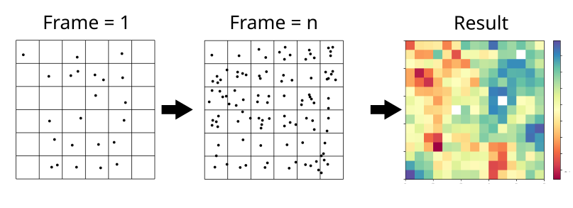
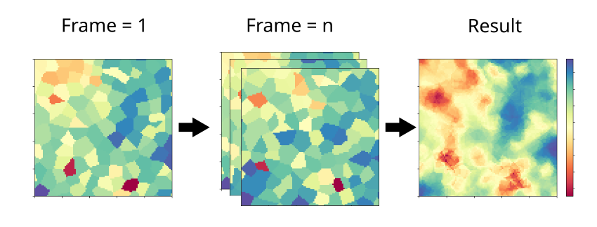
Cumulative2D projects membranes properties to the two dimensional plane of the membrane surface, perpendicular to the z axis.
The image below illustrates the protocol this class uses for the projection. The process begins by dividing the space into a \(m\times m\) grid. The xy positions of lipid phosphorus atoms and the respective analysis are collected over a user-set number of frames. These values are averaged within each grid square and stored in a \(m\times m\) matrix. Alongside this matrix, the grid edges are recorded in the format \([x_\text{min},x_\text{max},y_\text{min},y_\text{max}]\).
Note
The current version allows to select different number of bins for the x and y axis. The default is to use the same number of
bins for both axes. You can control this by passing a list of two values to nbins parameter. For example, to set
50 bins for the x axis and 100 for the y axis, use nbins = [50, 100]. If you pass an integer, it will be used for both axes.
To import Cumulative2D, type:
import MDAnalysis as mda
import numpy as np
import matplotlib.pyplot as plt
from twodanalysis import Cumulative2D
To use the class, call it using mda.AtomGroup or a mda.Universe as follows:
tpr = "md_membrane_nowater.tpr" # Replace with your tpr or gro file
xtc = "md_membrane_nowater.xtc" # Replace with your xtc file

universe = mda.Universe(tpr,xtc) # Define a universe

membrane = Cumulative2D(universe,   # load the universe
                verbose = False, # Does not print intial information
                nbins = 50)
Note
If your trajectory contains water and/or ions, pass the list of lipids in the membrane by specifying lipid_list.
Membrane Thickness
This code requires the user to set the number of bins, the edges, and the time interval. Additional options are listed in the documentation.
mat_thi, edges = membrane.thickness(50,           # nbins
                                    start = 61,   # Initial frame
                                    final = 110,  # Final Frame
                                    step = 1     # Frames to skip
                                    )
- The output is a matrix \(nbins\times nbins\) and the edges in the form
\([x_\text{min},x_\text{max},y_\text{min},y_\text{max}]\).
To visualize with plt.imshow:
import matplotlib.pyplot as plt

plt.imshow(mat_thi, extent=edges, cmap="Spectral")
plt.xlabel("x $\AA$")
plt.ylabel("y $\AA$")
plt.title("Membrane thichness from frames 61-110")
cbar = plt.colorbar()
cbar.set_label('Thickness $\AA$')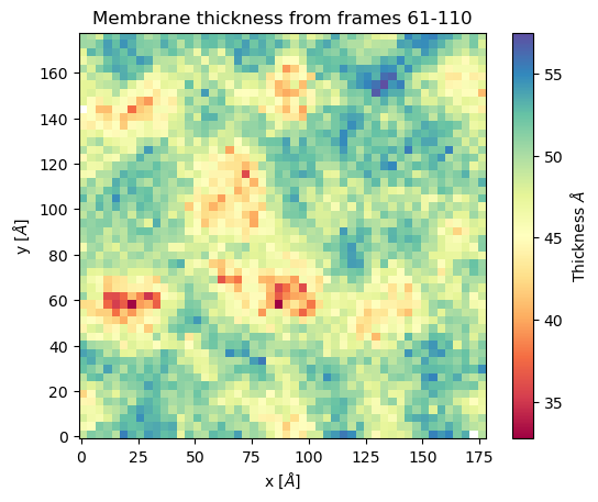
Membrane order parameters
To compute the order parameters the user must select the leaflet for which to run the analysis (top, bottom, or both) as shown below.
scd_top, edges = membrane.all_lip_order("top",
                                            50,
                                            start = 61,
                                            final=110,
                                            step = 1)
scd_bot, edges = membrane.all_lip_order("bot",
                                            50,
                                            start = 61,
                                            final=110,
                                            step = 1)
To plot the results:
from mpl_toolkits.axes_grid1 import make_axes_locatable
# Plot
fig, ax = plt.subplots(1,2, sharex = True, sharey = True)
first = ax[0].imshow(scd_top, extent=edges, cmap="Spectral")
ax[0].set_xlabel("x $\AA$")
ax[0].set_ylabel("y $\AA$")
ax[0].set_title("Top layer")
divider1 = make_axes_locatable(ax[0])
cax1 = divider1.append_axes("right", size="5%", pad=0.05)
cbar = fig.colorbar(first, cax = cax1)
# Point to a low ordered region
ax[0].add_patch(patches.Rectangle((48, 98), 20,20, linewidth = 1, edgecolor = "black", facecolor = "none"))
# High ordered region
ax[0].add_patch(patches.Rectangle((90, 120), 20,20, linewidth = 1, edgecolor = "black", facecolor = "none"))


second = ax[1].imshow(scd_bot, extent=edges, cmap="Spectral")
ax[1].set_xlabel("x $\AA$")
ax[1].set_title("Bot layer")
divider2 = make_axes_locatable(ax[1])
cax2 = divider2.append_axes("right", size="5%", pad=0.05)
cbar = fig.colorbar(second, cax = cax2)
cbar.set_label('|SCD| $\AA$')
plt.show()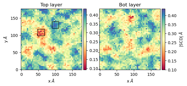
The image shows regions where the order parameters are low (in red) and high (in blue). Visual examination of those regions shows the lipids have the following configurations:

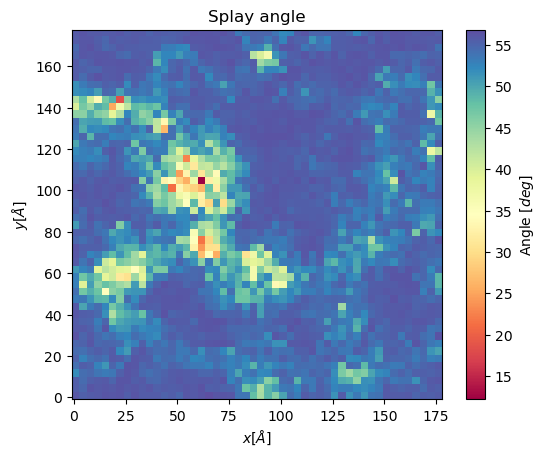
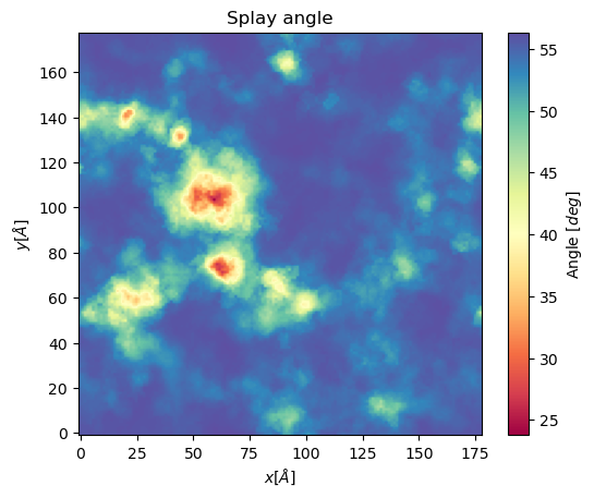
Splay Angle
The splay angle between lipid tails can also be projected to a 2D grid using Cumulative2D. To do so, the user defines two vectors from the lipid head (usually a P-atom) to the last carbons of the lipid tails, respectively. The angle between these vectors is mapped and averaged over the set number of frames to get the following plot.
splay, edges = membrane.splay_matrix(lipid_list = ["DSPC", "DODMA", "POPE"],
                                        layer = "top",
                                        nbins = 150,
                                        start = 61,
                                        final = 110,
                                        step = 1)
plt.imshow(splay, extent = edges, cmap = "Spectral")
plt.xlabel("$x [\AA]$")
plt.ylabel("$y [\AA]$")
plt.title("Splay angle")
cbar = plt.colorbar()
cbar.set_label('Angle $[\AA^2]$')
plt.show()
Voronoi2D
Voronoi2D also projects properties to a 2D grid, but using a different method.
Voronoi2D first constructs a Voronoi diagram using the positions of lipid head groups (typically lipid P-atoms), and mapping
them into a \(m\times m\) grid. The mapping step is done on each frame as illustrated in the figure below, and averages computed
across n frames. At each step, the value of the computed property is assigned to the grid squares that correspond to the xy position
of each lipid. The output, similar to Cumulative2D, is a matrix \(m \times m\), along with the
edges \([x_{\text{min}}, x_{\text{max}}, y_{\text{min}}, y_{\text{max}}]\).
Note
The current version allows to select different number of bins for the x and y axis. The default is to use the same number of
bins for both axes. You can control this by passing a list of two values to nbins parameter. For example, to set
50 bins for the x axis and 100 for the y axis, use nbins = [50, 100]. If you pass an integer, it will be used for both axes.
To import Voronoi2D type:
import MDAnalysis as mda
from twodanalysis import Voronoi2D
import matplotlib.pyplot as plt
Call the class using an mda.AtomGroup or mda.Universe as follows:
Note
The current version allows to select different number of bins for the x and y axis. The default is to use the same number of
bins for both axes. You can control this by passing a list of two values to nbins parameter. For example, to set
50 bins for the x axis and 100 for the y axis, use nbins = [50, 100]. If you pass an integer, it will be used for both axes.
membrane = Voronoi2D(universe, # load the universe
verbose = False, # Does not print initial information nbins = 100)
Note
If your trajectory contains water and/or ions, pass the list of lipids in the membrane by specifying lipid_list.
Membrane Thickness
The user must set the number of bins, the edges, and the time interval. Additional options are available in the documentation.
lipids = membrane.lipid_list.copy()
lipids.remove("CHL1")
mat_thi, edges = membrane.voronoi_thickness(lipid_list=lipids,
                                        nbins = 150,           # nbins
                                        start = 61,   # Initial frame
                                        final = 110,  # Final Frame
                                        step = 1     # Frames to skip
                                        )
The output is a matrix \(nbins\times nbins\) and the edges in the form \([x_{\text{min}}, x_{\text{max}}, y_{\text{min}}, y_{\text{max}}]\).
Visualize the output with plt.imshow:
import matplotlib.pyplot as plt

plt.imshow(mat_thi, extent = edges, cmap = "Spectral")

plt.xlabel("x $[\AA]$")
plt.ylabel("y $[\AA]$")

plt.title("Membrane thickness from frames 61-110")
cbar = plt.colorbar()
cbar.set_label('Thickness $\AA$')
plt.show()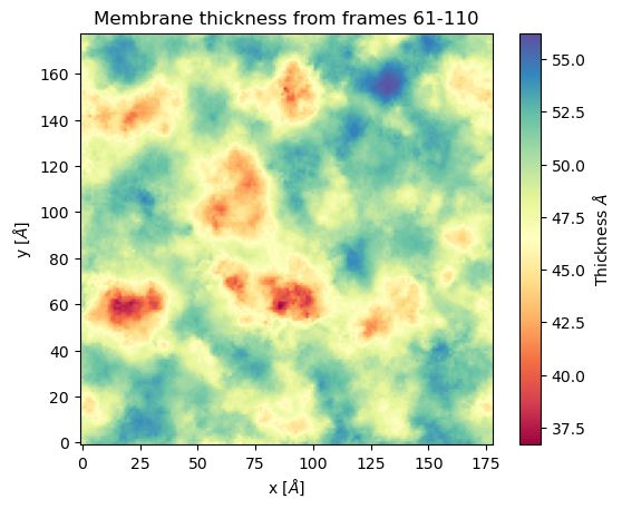
Area per lipid
The area per lipid (APL) is a metric of lipid lateral packingm typically used to determine thermal equilibrium of a lipid bilayer. This code plots the Voronoi APL for a single frame, output images can be merged into a giff or short movies.
To run this analysis type:
voronoi_dict = membrane.voronoi_properties(layer = "top")
This will return a dictionary that contains the APL per residue in the top bilayer, accesible as voronoi_dict["apl"].
To map the Voronoi APL and compute its mean over time use:
areas, edges = membrane.voronoi_apl(layer = "top",
                                    nbins = 150,
                                    start = 61,
                                    final = 110,
                                    step = 1)
To render the plot use:
plt.imshow(areas, extent = edges, cmap = "Spectral")
plt.xlabel("$x [\AA]$")
plt.ylabel("$y [\AA]$")
plt.title("Area per lipid")
cbar = plt.colorbar()
cbar.set_label('Area per lipid $[\AA^2]$')
plt.show()

Splay Angle
Voronoi2D can also project the splay angle between lipid tails to a 2D grid. Similar to Cumulative2D, the user must set the two vectors that define the lipid tails. Using the Voronoi2D protocol, the splay angle is plot for a set number of frames as follows.
splay, edges = membrane.voronoi_splay(layer = "top",
                                        nbins = 150,
                                        start = 61,
                                        final = 110,
                                        step = 1)
plt.imshow(splay, extent = edges, cmap = "Spectral")
plt.xlabel("$x [\AA]$")
plt.ylabel("$y [\AA]$")
plt.title("Splay angle")
cbar = plt.colorbar()
cbar.set_label('Angle $[\AA^2]$')
plt.show()
PackingDefects
The membrane surface topology is highly dynamic, different lipid species and interactions with other biomolecules result in local changes that can be identified using 2Danalysis methods. Lipid packing defects analysis is used to quantify the exposure of the hydrophobic membrane core. PackingDefects code allows efficient and robust statistical analysis of lipid packing deffects on the membrane surface. The analysis can be done for a single frame as well as for the full trajectory.
Import this class as follows:
import MDAnalysis as mda
from twodanalysis import PackingDefects
Call the class using an mda.AtomGroup or mda.Universe as follows:
tpr = "mlkl_membrane.gro" # Replace with your tpr or gro file
xtc = "mlkl_membrane.xtc" # Replace with your xtc file

universe = mda.Universe(tpr,xtc) # Define a universe with the trajectories

membrane = PackingDefects(universe,   # load the universe
                verbose = False # Does not print intial information
                )
Single Frame
To run the analysis for a single frame, set the frame number of interest and run:
membrane.u.trajectory[100] # Compute deffects for the 80 frame
defects, defects_dict = membrane.packing_defects(layer = "top",         # layer to compute packing defects
                                                periodic = True,  # edges for output
                                                nbins = 400            # number of bins
                                                )
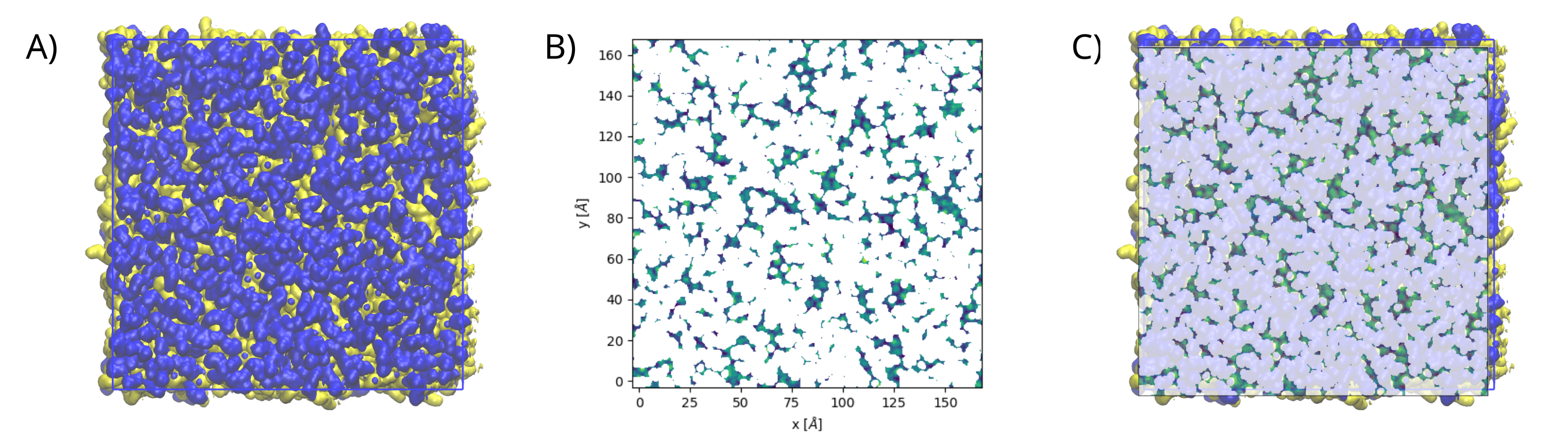
To plot and visualize the output run:
plt.imshow(defects, cmap = "viridis", extent = defects_dict["edges"]) # Plot defects
plt.xlabel("x  $[\AA]$")
plt.ylabel("y  $[\AA]$")
plt.show()

The following figure shows: (A) the packing deffects plot on VMD, (B) the output from PackingDefects, and (C)
the overlay of both approaches for comparison and validation
Multiple Frames
For statistical analysis of packing deffects across several frames, PackingDefects returns a pandas dataframe
and an array with the size of individual packing defects along the trajectory.
To run the analysis over n frames type:
data_df, numpy_sizes = membrane.packing_defects_stats(nbins = 400,
                                                  layer = "top",
                                                  periodic = True,
                                                  start = 0,
                                                  final = -1,
                                                  step=1)
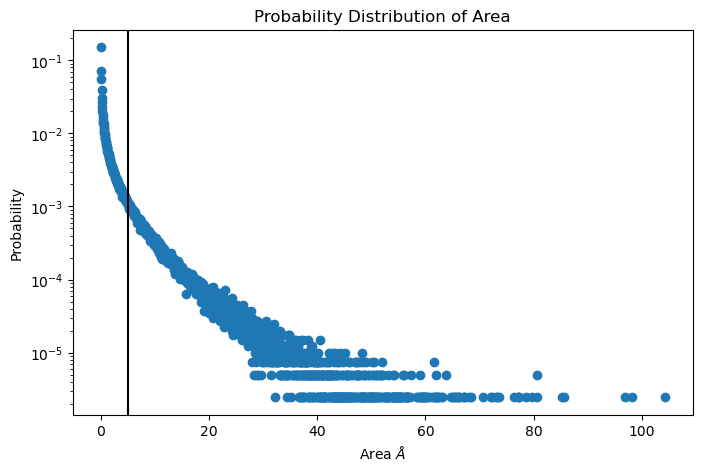
To plot the distribution of packing defects areas type:
unique, counts = np.unique(numpy_sizes, return_counts = True)
probabilities = counts/counts.sum()

plt.figure(figsize=(8, 5))
plt.scatter(unique*defects_dict["grid_size"]*defects_dict["grid_size"], probabilities)
plt.xlabel('Area $\AA$')
plt.yscale('log')
plt.ylabel('Probability')
plt.title('Probability Distribution of Area')
plt.axvline(x = 5, color = "black")
plt.show()
BioPolymer2D
This quick user guide includes instructions on how compute the following analysis:
Polar histogram analysis
2D position density contours
Parallel and perpendicular radii of gyrations
Hydrogen bonds per residues
Download trajectory files
Although this quick guide is designed to be adapted to work with any trajectory, it is strongly recommended to first follow it using our trajectories to gain an initial approach to the parameters you need to adjust and how to modify them for your own system.
To proceed, download our trajectories from Zenodo using the wget command (if needed, install
it with pip install wget in the command line). The download may take a few minutes. A directory
named data will be created containing the downloaded trajectories.
import wget
import os
url_tpr = 'https://zenodo.org/records/14834110/files/md_biopolymer_nowater.tpr'
url_xtc = 'https://zenodo.org/records/14834110/files/md_biopolymer_nowater.xtc'
os.makedirs('data', exist_ok=True)
load_MD_NOWATER_TPR = wget.download(url_tpr,out='data/md_biopolymer_nowater.tpr')
load_MD_TRAJ = wget.download(url_xtc,out='data/md_biopolymer_nowater.xtc')
Before we start the analysis, we need to import MDAnalysis (since our class is initialized with a
MDAnalysis AtomGroup or Universe), and our class.
import MDAnalysis as mda
import matplotlib.pyplot as plt
from twodanalysis import BioPolymer2D
We initialize our object using a MDAnalysis Universe, or a AtomGroup, and the selection of the surface inteface. Although, selecting the surface interface is not mandatory it is highly recomended. In particular, if you expect to make polar histograms or any of the 2D density contour plot.
MD_NOWATER_TPR='data/md_biopolymer_nowater.tpr' # Replace this with you own topology file
MD_TRAJ='data/md_biopolymer_nowater.xtc' # Replace this with your trajectory file

universe = mda.Universe(MD_NOWATER_TPR,MD_TRAJ) # Define a universe with the trajectories
sel=universe.select_atoms("protein") # Use any convinient selection.

biopol = BioPolymer2D(sel, surf_selection='resname DOL and name O1 and prop z > 16')   # Initialize object by loading selection.
If BioPolymer2D is initialized with a Universe, the whole universe is considered to be the selection.
We can also set our biopolymer to be subset of the mda.Universe or mda.AtomGroup by adding the input parameter
biopol_selection with a subset selection. Note that the biopolymer is not necesarilly a protein but
can also be a nucleic acid.
Note
Polar histograms and the 2D density contour analyses use two parameters to filter frames where the biopolymer object is desorbed:
zlim: Sets the minimal distance (in \(\mathring{\text{A}}\)) residues need to have to the surface to be considered absorbed, e.i filters frames where \(\langle z_i\rangle_{\text{residues}}\) >zlim.Nframes: Sets the number of frames to consider from the set of \(\langle z_i\rangle_{\text{residues}}\) <zlimframes. IfNframes=None, it considers all frames.
zlim will take as reference of the surface the mean value over time and atoms of the selected surface interface atoms selected at the initialization of the object (surf_selection input parameter).
For this reason is importante that surf_selection selects only the atoms at the interface of the surface rather that the whole surface.
If we want to consider only a set of frames (or times) of the whole trajectory, we can initialize as,for instance,
biopol = BioPolymer2D(sel, surf_selection='resname DOL and name O1 and prop z > 16',start=100,step=2,end=300)
By default start, step, and end are parameters set in frames. If we rather set these parameters in time units (in ns), we can add by_frames=False as a input parameter.
These 3 parameters can be set independently (do not need to set them three if only one is wanted to be modified).
With INFO method we can retreive general information on our universe and selection, and we can set a system name with system_name
attribute. Especially convinient if working with more than object at the same time, since the names will appear in the legends.
biopol.system_name='Omicron PBL1'
biopol.INFO()
In general, we would also like to compute the positions of the residues in our object. This will store position values of each frame
of the center of mass (COM) of the residues of all its atoms on the pos attribute. Compute:
biopol.getPositions()
If you want to consider different set of frames than those used at the initialization of the object, The attributes startT, endT, and stepT
(for setting times) or startF, endF, and stepF can be overwriten before computing getPositions,e.g.
biopol.startT=100
biopol.endT=200
biopol.stepT=1
biopol.INFO()
biopol.getPositions()
INFO to confirm that startT, endT, and stepT have been overwriten.
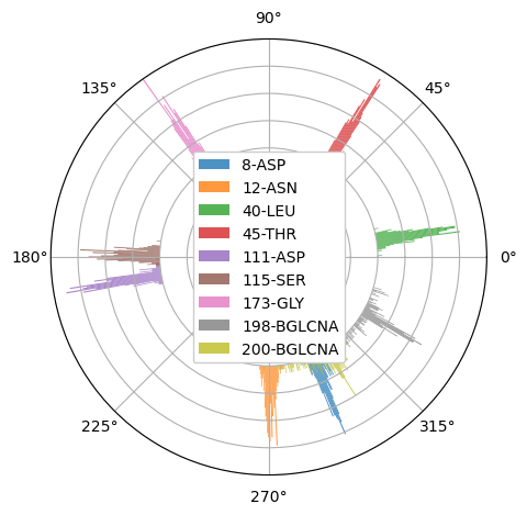
Polar histogram analysis
Since we are interested in only sampling the adsorption, PolarAnalysis method filters the frames in which the object is not
adsorbed using a zlim and Nframes parameters. Frames in which minium position of residues in our select_res selection is lower than zlim to the surface,
are considered adsorbed.
Now, in general, the number of adsorbed frames will vary for different trajectories, and ,if we want to compare results between trajectories,
Nframes paramater will set the number of frames we want to take from the total adsorbed frames, taking the Nframes frames where our
select_res selection is most adsorbed to be sampled in the histograms.
We compute the PolarAnalysis, setting these parameters,
select_res='resid 198 200 12 8 40 45 111 115 173'
zlim=15
Nframes=900
hist_arr,pos_hist=biopol.PolarAnalysis(select_res,Nframes,
                                            zlim=zlim,control_plots=False,plot=True)
plt.show()
If we only want to compute the histogram, and don’t want any plot, we can set plot=False. control_plots is to visualize the different steps of the PolarAnalysis calculations.
Titles and further figure customization can be added to the plot using standard matplotlib.pyplot methods before plt.show().
Warning
If ``surf_selection`` input parameter was not set in the object initialization, the surface in the trajectory will not set the z=0, and zlim will not
work correctly, since it expects the surface intefarce with the protein to be the reference.
We suggest overwriting the surf_pos attribute with the position of the surface (<0,x,y,z> format) before computing the PolarAnalysis method.
Only the z value will be used.
surface_selection='resname DOL and name O1 and prop z > 16'
surface_pos=biopol.getPositions(select=surface_selection, inplace=False)
biopol.surf_pos=surface_pos
With the inplace=False it will not overwrite the pos attribute of the object, but only return it.
2D position density contours
In general, we would like to have a reference of the position of the whole biopolymer to have insight ont the flexible regions. Therefore, we first compute the KDE of whole molecule, and then compute the KDE of selected residues:
paths=biopol.getKDEAnalysis(zlim,Nframes,) # Computes the paths of all the contour levels
biopol.plotPathsInLevel(paths,0,show=False) # Plots paths in contour level 0
# Plot the KDE contour plots of the selected residues
all_residues_paths,residues_in_contour=biopol.KDEAnalysisSelection('resid 198 200 12 8 40 45 111 115 173',Nframes,zlim,show=False,legend=True)
plt.show() # Can also set "show=True" if no plot customization is required.
Note
Setting the same zlim and Nframes paramater values for PolarAnalysis , getKDEAnalysis and KDEAnalysisSelection is suggested.
We now can compute the Areas of the paths computed by KDEAnalysisSelection with the getAreas attribute as follows:
data=[]
for p in range(len(all_residues_paths)):
    areas=BioPolymer2D.getAreas(all_residues_paths[p],0,getTotal=True) # Stores the total area of contour level 0.
    data.append([residues_in_contour.residues[p].resid,residues_in_contour.residues[p].resname,areas])
df=pd.DataFrame(data=data, columns=["ResIDs", "Resnames", "Area (angs^2)"])
df
df will show a table with the areas of the outer contour levels (level 0 in getAreas , is outer).
Parallel and perpendicular radii of gyrations
The parallel and perpendicular radii of gyration gives structural information during the adsorption,
\(R_{g\parallel}\): Gives information on how the biopolymer is expanded by the sides (parallel to the surface).
\(R_{g\perp}\) : Gives information on how the biopolymer is streched or flattened.
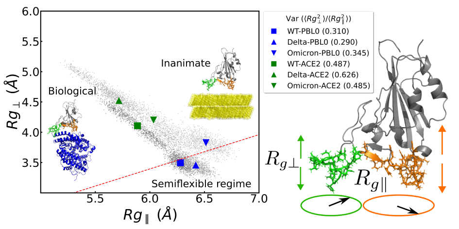
Figure 1: Example of radii of gyration correlation figures that can be made with method on the left and a schematic representacion of the parallel and perpendicular radii of gyrations on the right. Figure taken from the TOC figure of Bosch et. al (2024).
To notice significant results, we need to select a region that is in contact with the surface as our object, e.g.
sel_in_Contact=universe.select_atoms('resid 4-15 or resid 34-45 or resid 104-117 or resid 170-176') # Select region in contact with surface
Contact_region = BioPolymer2D(sel_in_Contact, surf_selection='resname DOL and name O1 and prop z > 16') # Initialize object
Contact_region.system_name='Contact Omicron PBL1'# Set system name
Contact_region.getPositions() # Compute positions
ratio=Contact_region.RgPerpvsRgsPar(rgs, 'tab:green',show=False) # Make RgPerp vs Rg parallel plot
The output will be similar to Figure 1 (left), with only one system instead of six. Also, by default, small dot will be colored (and will represent the
\(R_{g\perp}\) and \(R_{g\parallel}\) values at each frame), and bigger markers will be black (representing the mean values of the data).
Example of this can be seen in BioPolymer2D Tutorial .
The ratio will give the \(\langle R_{g\perp}^2 \rangle /\langle R_{g\parallel}^2 \rangle\) ratio, which is relevant on charactertizing the adsorption of polymers
(Egorov et. al (2016)`, Milchev et. al (2020), Poblete et. al (2021)).
Hydrogen bonds per residues
To the hydrogen bonds between two arbitrary selections of residues. In particular, you can compute the hydrogen bonds present between a biopolymer and a the surface as follows:
select_biopol='protein or resname AFUC BMAN AMAN BGLCNA' # Selection of protein and its glycan
select_surf='resname DOL' # Selection of atoms present in the surfaces
biopol.getHbonds(select_surf,select_biopol) # Compute H-bonds between surface and biopolymer
By default, the H-bond count will be stored in the attribute hbonds of the object, which can be changed to only returning the result setting
inplace=False in getHonds.
To visualize these results, we suggest using the plotHbondsPerResidues method. Previous to use this method, you will need to compute a KDE contour plot
plot as a reference of the biopolymer.
paths=biopol.getKDEAnalysis(zlim,Nframes)
biopol.plotHbondsPerResidues(paths,contour_lvls_to_plot=[0,5,8],top=5, print_table=True)
plt.show()
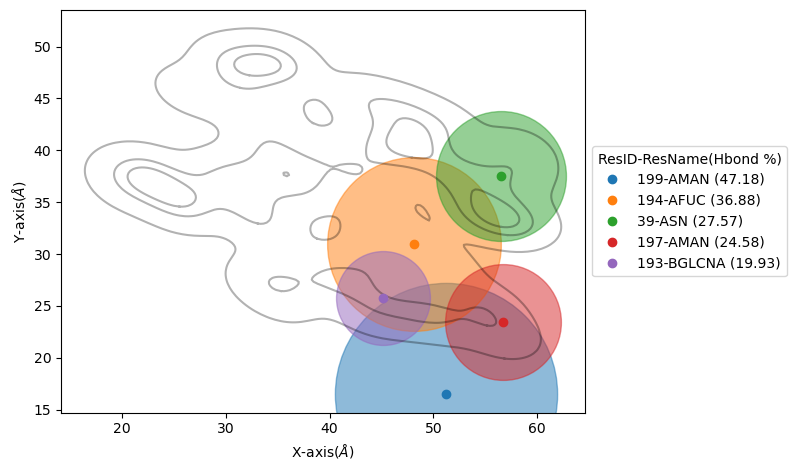
Here, you will be showing the contour levels 0 (outer), 5 (middle) and 8 (inner) as reference. Also, you will be plotting only the 5 residues with
most H-bonds during the simulation (using top paramater), and with print_table we are setting to print a table with all the residues with their H-bond
percentages during the simulation (note that these percentagesare shown for our top residues in the legend). We can add the filter input parameter to remove residue names we are not interested
to see on the plot.
References